Grouped Reports in Excel Using Power Query

One of my favourite Airtable features is the option to group records in a grid view. It’s such a simple and effective way of organizing information and getting helpful summary info with per-group subtotals. However, now that Airtable is blocked by the firewall at work, I’ve been having to make do with pivot tables or manually grouping data into sections in Excel.

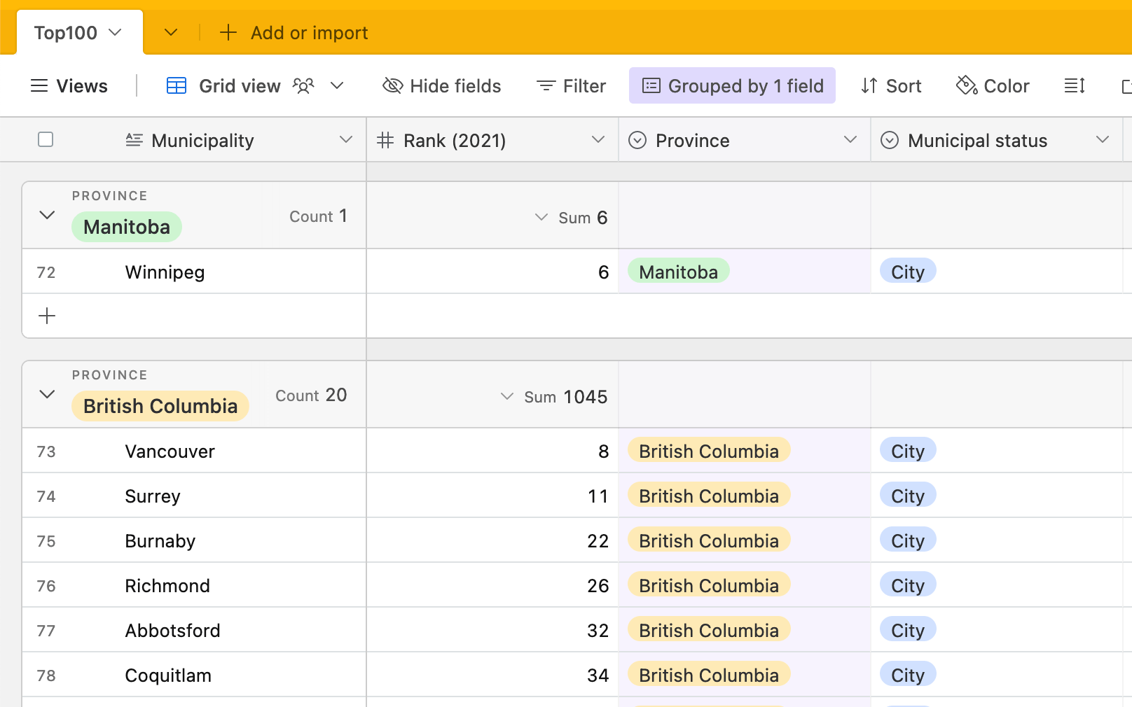
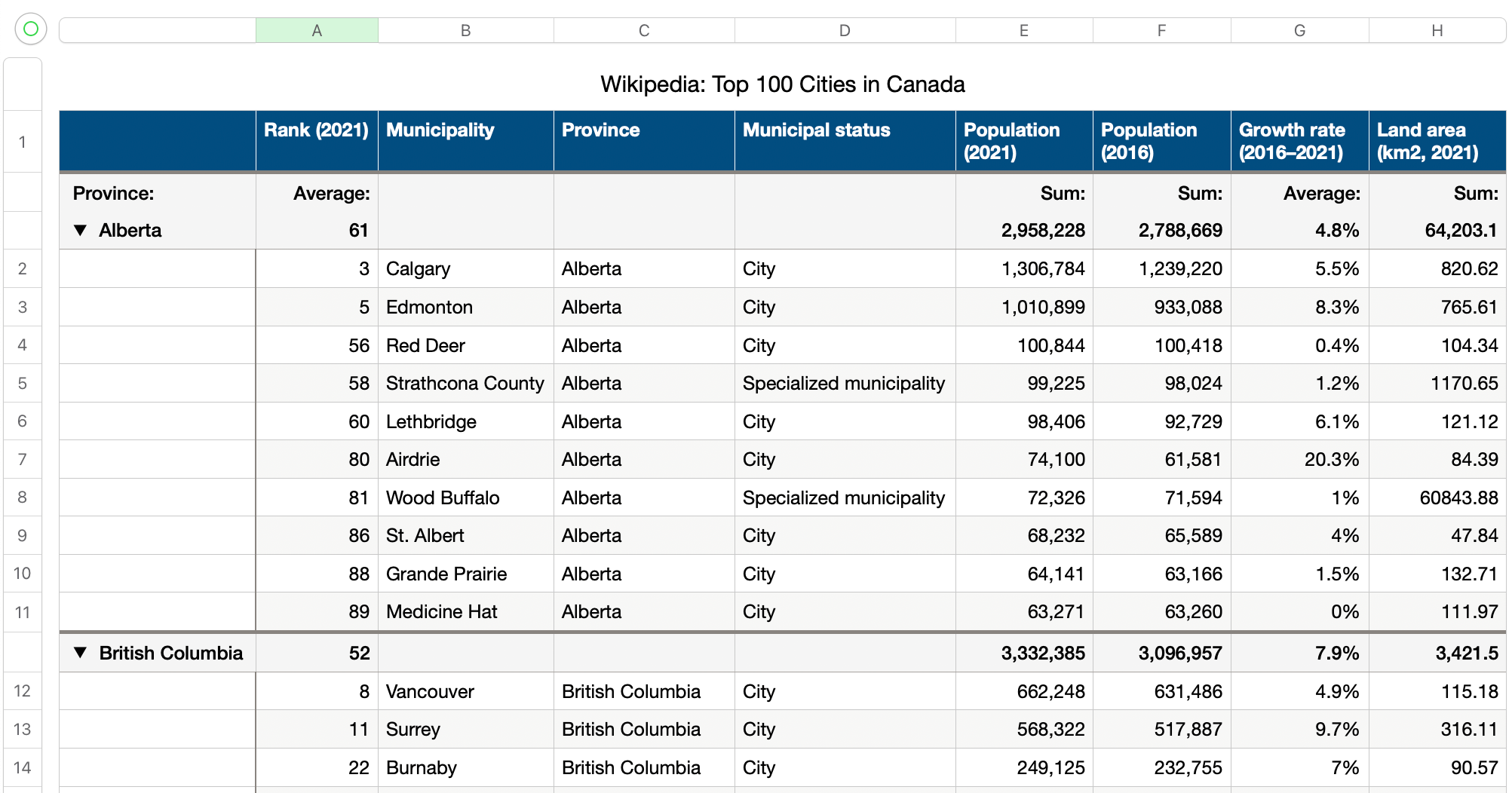
An example of grouped records in Airtable

Sadly, Excel is way behind when it comes to simple and useful grouping of data ¹. Although pivot tables are powerful, they have a terrible UI for custom styles, and can be pretty fiddly. Similarly, Excel’s “group data” features allow you to expand and collapse rows, but row groups don’t dynamically update as data changes, and require a lot of manual upkeep.

One Excel feature I do love (well, love-hate) is Power Query. It has some quirks, but it offers a lot of power when combined with named table ranges ². It’s a great way to take your existing data and merge tables together or pull a subset of data onto another sheet.

So I decided to try making grouped records using a custom Power Query formula ³, and it turned out pretty well! If you want to try it yourself, I’ve included the code and instructions below. Here’s a sneak peek at the final result:

Instructions

Get the Script

Get the code for the query formula on GitHub.

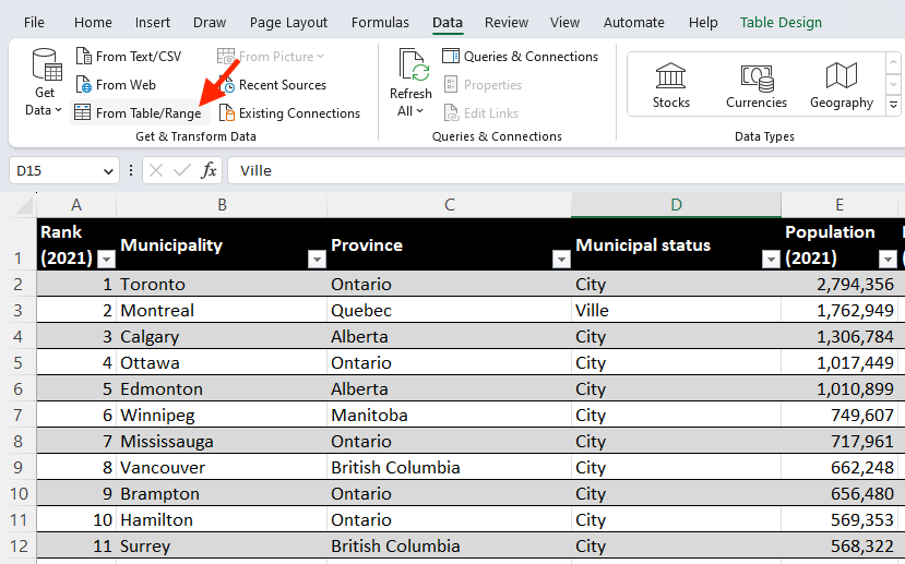
To use this query formula, you’ll need a named table with data that includes a column for your grouping category. For our example, we’ll use Wikipedia’s list of the largest municipalities in Canada.

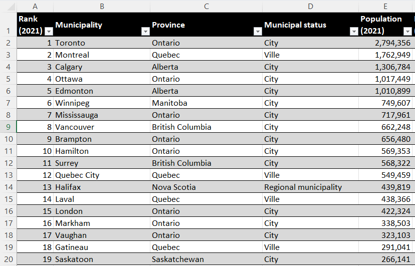
To make a grouped list of our data, first we’ll load the data into Power Query using Data > From Table/Range.

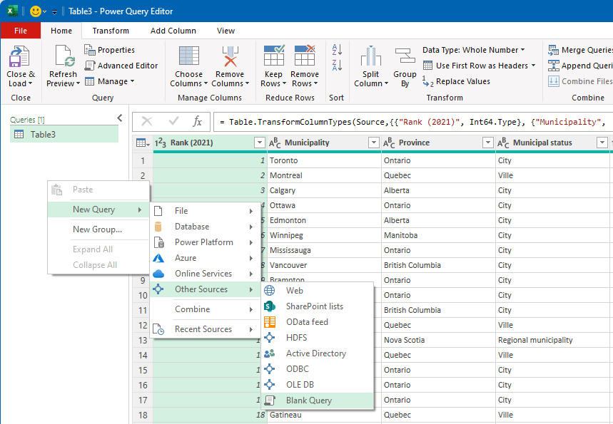
In the query editor, before we start transforming our data, we’ll first have to set up the custom function. On the left, right-click and then select New Query > Other Sources > Blank Query.

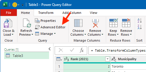
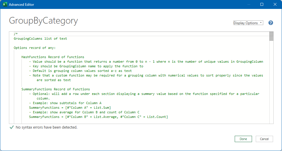
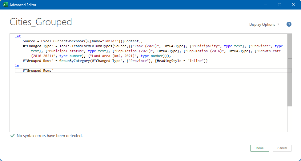
Rename your new blank query GroupByCategory ⁴, open the Advanced Editor, remove the placeholder text and paste in the script from Github.

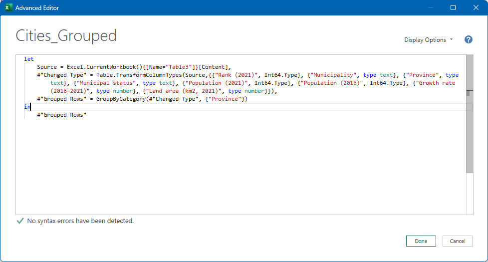
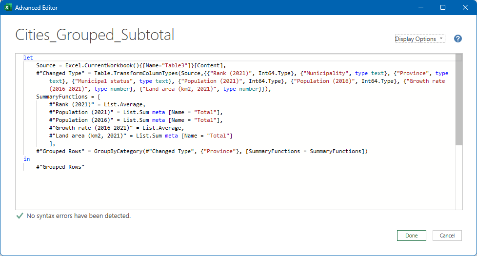
The pasted code should look something like this:

With the custom function set up, we can now go back and use it for the city data. In the city data query, open up the advanced editor and add in a new row as follows:

• Add a comma to the end of the last row before in.
• Just after that row (but still before the in keyword), add in #"Grouped Rows" = GroupByCategory(#"Changed Type", {"Province"})
• Change the last line to #"Grouped Rows".

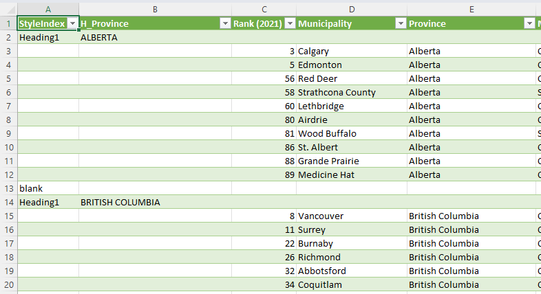
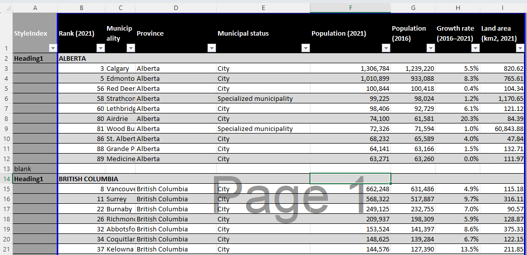
Now, you can select “Close & Load” and Excel will insert a new tab with your output table. It still needs some formatting work, but you can see it’s now grouped our data by province.

Wait, What Did I Just Do??

In case you haven’t used the advanced editor before, this is what’s happening — the code for Power Query transform operations is written in a format like this, with all lines in each section except for the last one separated by commas:

let
  Source = <<expression that loads in your data>>,
  #"Step A", // applies a transformation to Source
  #"Step B" // applies a transformation to #"Step A"
in
  #"Step B" // step you want the output from

When you use the Power Query menu to do things like remove or reorder columns, or change data types, the program generates this code behind the scenes. Occasionally, when you need to do something more complex, you have to edit the code directly, like we did here.

In our case, we added a step that calls our custom function GroupByCategory, which has two required arguments:

• The table you want it to process (in our case, the output from the #"Changed Type" step).
• A list of the names of the columns that should be used to group the data. In our case, there was only one item in our list, but you’ll see an example at the end of grouping by more than one column.

Our function then spits out a table with the data grouped, heading rows added, etc.

If you want to learn more about the code behind Power Query, you can read through the documentation for the Power Query M formula language, though be warned that it may be a bit challenging in places if you’re not familiar with computer programming jargon. If you search for “M Query Beginner” you’ll probably find some blogs and videos that have clearer and more example-based explanations.

Formatting Your Table

To make our table look a little more presentable, let’s format it a little bit.

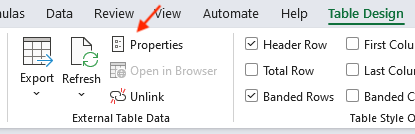
Before we dive in, let’s make sure we can manually control the column widths by changing the table properties. First, select any cell of the table, then select the “Properties” button in the “Table Design” section of the ribbon.

Uncheck “Adjust column width” and select OK.

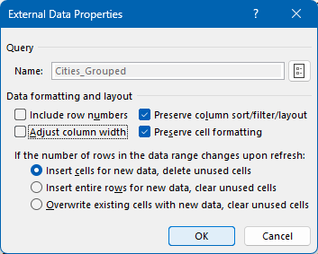
This will stop the table from auto-fitting the column widths when we refresh our data.

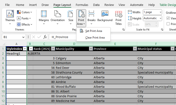
We also want to hide the StyleIndex column, which can be done by just hiding the column or by excluding it from the print area. To change the print area, select the columns you want to be printed, and then select Page Layout > Print Area > Set Print Area:

For the table itself, we can do some pretty simple formatting:

• Choose a different table colour scheme from the Table Design menu in the ribbon
• Resize the H_Province column to e.g. 3 units and hide the heading title by changing the text colour of B1 to match the background
• Apply some number formatting where needed (e.g. changing the Growth Rate column to percentages)

At the end, our table now looks something like this:

Inline Layout

By default, the function will output a table in “Outline” style with a new column added on the left for each grouping level. This gives some visual indentation and allows you to easily format the headings by formatting just the heading column.

However, you can also choose an “Inline” style where the headings are put in the first data column instead. To do this, we’re just going to add an option to our function call in the script using the optional third argument of the function, which lets us configure how the function works ⁵. Now our function line will look something like this:

#"Grouped Rows" = GroupByCategory(#"Changed Type", {"Province"}, [HeadingStyle = "Inline"])

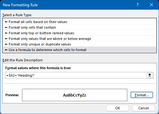
To get our bolded heading, we’re going to have to use some conditional formatting. With our table data selected, select Home > Conditional Formatting > Manage Rules > New Rule and set up a formula rule with the function set to =$A2="Heading1" (where $A2 is the first cell in the selected range). In this case, I’ve also set the text format for this rule to “bold”.

Our result should look something like this:

Note that for the Inline style, the group headings are in the first column (“Rank (2021)”) instead of in their own column to the left of the data.

The benefit of conditional formatting is that it should continue to work as intended, even as your table grows or shrinks. With everything set up, when you need to use the table, all you’ll need to do is refresh the data (Right-click table and select “Refresh” or Data > Refresh All in the ribbon).

Adding Summary Functions

In many cases, it’s also helpful to have automatic subtotals for certain columns show for each group. Let’s set that up now.

Go back into the query editor (Data > Queries & Connections > Right-Click and select “Edit”), open up the Advanced Editor again and add in the following line and function option:

SummaryFunctions = [
  #"Rank (2021)" = List.Average,
  #"Population (2021)" = List.Sum meta [Name = "Total"],
  #"Population (2016)" = List.Sum meta [Name = "Total"],
  #"Growth rate (2016-2021)" = List.Average,
  #"Land area (km2, 2021)" = List.Sum meta [Name = "Total"]
  ],
#"Grouped Rows" = GroupByCategory (#"Changed Type", 
  {"Province"}, [SummaryFunctions = SummaryFunctions])

What we’ve done here is define a Record of summary functions to apply to specific columns, and provided that Record as an option for our function.

By default, the function will also add in a row at the top with labels for the summary functions so that it’s clear which column has averages vs totals, etc. For the built in List functions the name comes from the function itself, e.g. List.Sum would be labeled “Sum”. However, you can provide your own labels by adding a metadata field Name like you can see in the example above, where we want our Sum functions to be labeled “Total” instead. The metadata label can also be used if you want to use your own custom functions for summarizing a column.

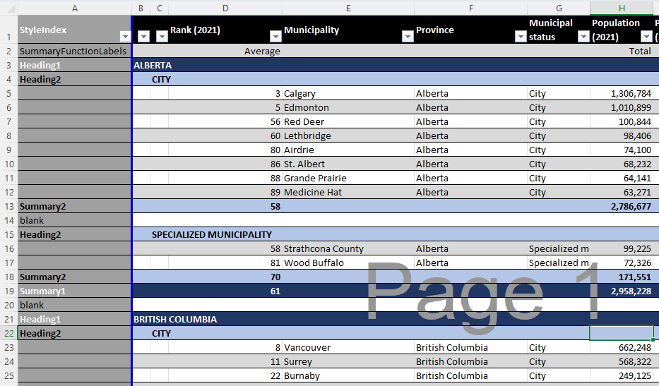
Here’s what the output will look like (with some additional steps we’ll get into just below) — you can see we have per-group averages for the Rank column and per-group subtotals for the Population column.

Grouping by Multiple Columns

You might have also noticed in the example above that we have multiple groups, with the data grouped by Province, and then within each Province by Municipal Status.

To set this up, we just have to make a small change to our function line in the code so that we list both our grouping columns in the desired order:

#"Grouped Rows" = GroupByCategory (#"Changed Type", 
  {"Province", "Municipal status"}, 
  [SummaryFunctions = SummaryFunctions]
  )

This will now give us heading and summary rows for each grouping column, so let’s set up some more advanced conditional formatting to make the data structure clearer:

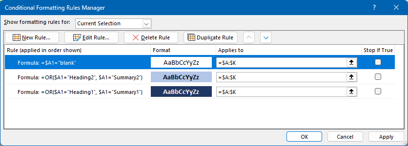
(In this case, I’ve selected entire columns instead of just the table data, so the first cell in my range is $A1).

Also, it’s not obvious from the formatting options in the screenshot above, but the blank rows have a white background applied to override the alternating colours from the table style.

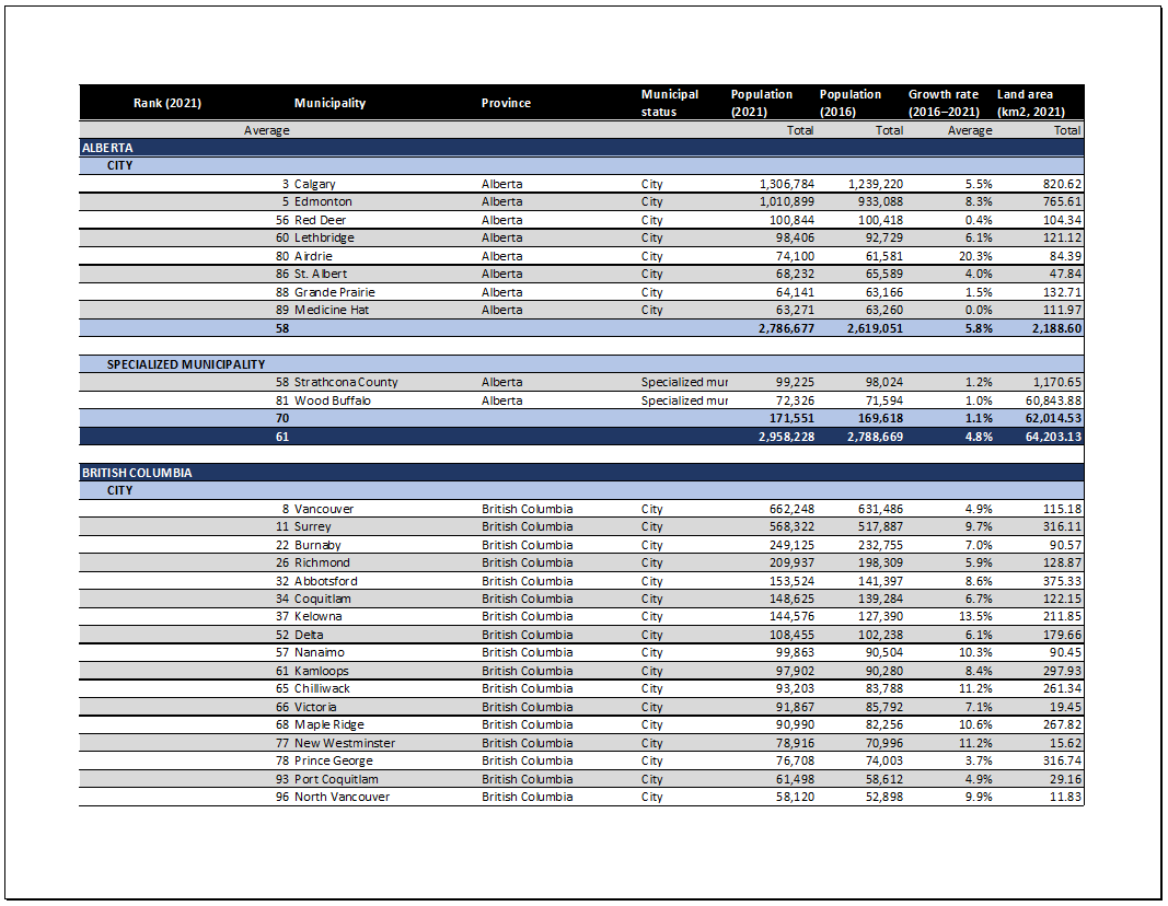
This should now be everything we need to get our formatted, multi-grouped table:

Some Printing Tips

In addition to hiding the StyleIndex column or excluding it from the print area, there are two small details you may want to set up if you want to print your table or save it to PDF:

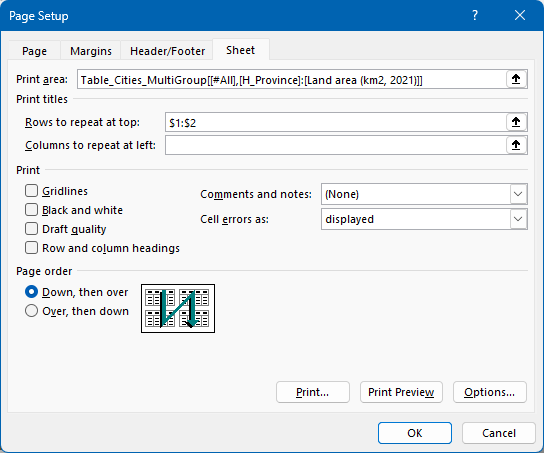
First, you can have the heading row and summary function labels repeat on each page by going to Page Layout > Page Setup > Sheet and selecting these rows using the “Rows to repeat at top” control.

Second, in the Page Layout section of the ribbon, you may also want to change the page orientation to Landscape and set the Width to 1 Page if you have a lot of columns and want them all on the same page.

Finally, after you’ve refreshed your table data, you may want to adjust where the page breaks are by selecting the page break preview in the view options on the bottom-right hand corner of the application window (next to the zoom control). Once you’re in Page Break Preview, you can drag the break lines up as needed. If you ever need to reset the breaks and set them again from scratch, go to Page Layout > Breaks > Reset All Page Breaks.

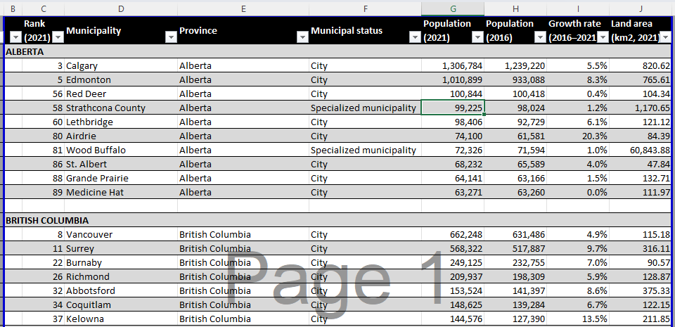
With these options applied, you’ll have a print output that looks something like this:

Final Thoughts

This process may feel like a lot of steps, especially if you’ve never used many of these Excel features before. However, compared to setting up a grouped report in Microsoft Access or the Power BI Report Builder, using this custom function will be a lot easier for many people.

For simpler cases, Pivot Tables might be a more straightforward solution, though I’ve often found them incredibly frustrating to format.

If you really want to have some fun, you can also set up another table to specify your grouping columns and make your sheet into more of an interactive report generator. I’ll leave that as an exercise for the reader.

There are still some unavoidable drawbacks to using Excel instead of Airtable. For example, you can’t edit your data directly in the grouped output table, and Excel for Mac doesn’t quite have the same number of Power Query features as the Windows version (though it’s quickly catching up).

However, when Excel is the tool you need to use, I think this is a useful tool to have. I hope you find it useful too! If you run into any bugs or issues, make sure to flag them on the Github Issues Page.

1. Hot take: this use case is something that Apple Numbers is actually better at than Excel. See: Modify category groups in Numbers on Mac and Add calculations to category groups in Numbers on Mac.

    ↩

2. For those that don’t know, you can take a named table range, select “From Table/Range” in the Data tab, and then “Close & Load To…” with the option to “Only Create Connection”. This sets up a query for your table data that you can then reference in other queries, e.g. via “Merge Queries”. ↩

3. Shout out to this great post by Livio on XcelanZ.com which helped me figure out how to code in the blank rows between sections. ↩

4. Because the function is recursive, if you want to use another name, you’ll also have to change the @GroupByCategory reference near the end of the script to match your function name. ↩

5. The full list of options can be found in the mega-comment at the top of the function script itself. ↩